Probabilistic hyperbolic embedding of networks
Combining network geometry with Bayesian inference
2025-05-06
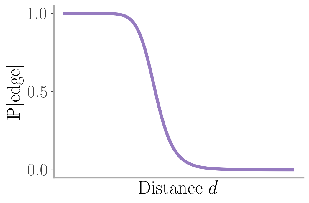
Creating edges requires a cost
Vertices are placed in metric space. The edge cost increases with its length.

The metric space can be physical (e.g. transportation network, brain network) or not.
Latent hyperbolic space
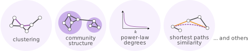
Graphs obtained from hyperbolic space reproduce many empirically observed properties.
Krioukov, D., et al. Hyperbolic geometry of complex networks. Phys. Rev. E 82, 036106 (2010).
Zuev, K., et al. Emergence of Soft Communities from Geometric Preferential Attachment. Sci. Rep. 5, 9421 (2015).
Krioukov, D., et al. Clustering Implies Geometry in Networks. Phys. Rev. Lett. 116, 208302 (2016).
- Faqeeh, A., et al. Characterizing the Analogy Between Hyperbolic Embedding and Community Structure of Complex Networks. Phys. Rev. Lett. 121, 098301 (2018).
Graph vertex embedding in a nutshell
We want to represent a given graph using a hyperbolic embedding.
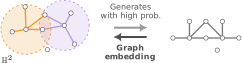
This amounts to:
\[ \text{Pairs of vertices are} \begin{cases} \text{close} & \text{if connected in graph,} \\ \text{far} & \text{if not connected in graph.} \\ \end{cases} \]
Embedding with maximum likelihood
The likelihood of obtaining a graph \(G=(V, E)\) is simply \[\begin{align} \mathbb{P}[G|\theta, \kappa, \beta] = \prod_{(u, v)\in V^2} {p_{uv}}^{a_{uv}} (1-p_{uv})^{1-a_{uv}}, \end{align}\] where \(a_{uv}=1\) if \(u\) and \(v\) are connected and is \(0\) otherwise.
Many algorithms give a maximum likelihood estimator (MLE). This is challenging because of the abundance of local maxima.
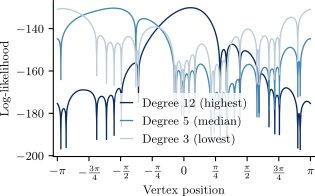
\(\mathbb{S}^1\) Bayesian model
The posterior of the Bayesian \(\mathbb{S}^1\) model is \[\begin{align} p(\theta, \kappa, \beta | G) \propto \mathbb{P}[G|\theta, \kappa, \beta] \; p(\beta) \prod_{v \in V} p(\theta_v)p(\kappa_v), \end{align}\] where the priors are
\[\begin{align} \theta_u &\sim \text{Uniform}[-\pi, \pi), \\ \kappa_u &\sim \text{Cauchy}, \quad \kappa_u >\epsilon,\\ \beta &\sim \text{Normal}, \quad \beta>1. \end{align}\]
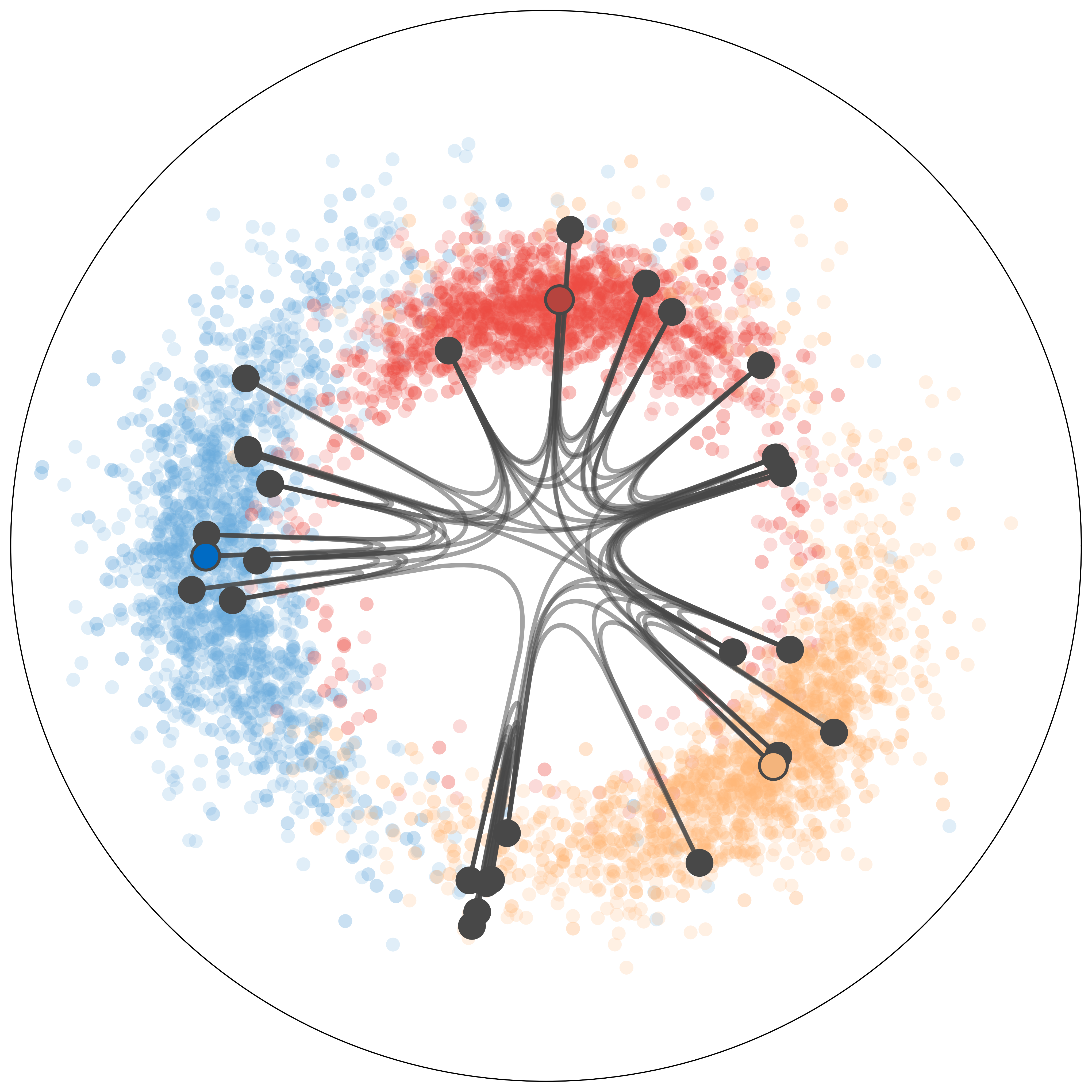
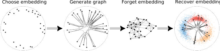
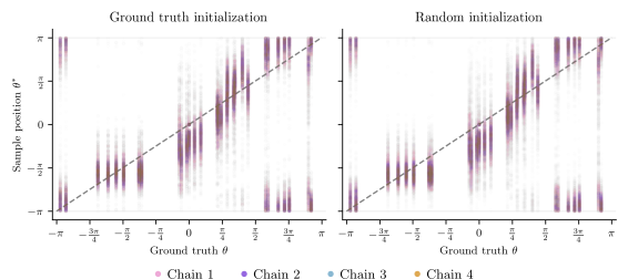
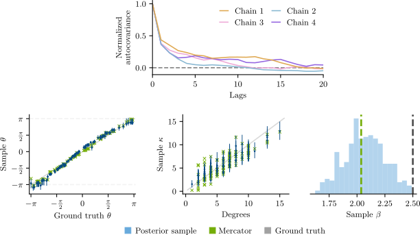
Sanity check with synthetic data
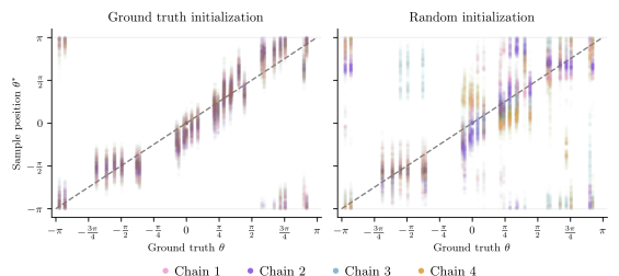
Usual sampling methods don’t work
Hamiltonian Monte Carlo1 (HMC) and random walk don’t sample properly.
Locality implies clusters
Since edges are local, groups of nearby vertices should be moved together.
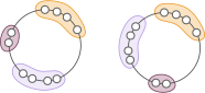

Cluster transformations fix the sampling issue
Cluster transformations + random walk yield good samples of the posterior.
Embedding error bars
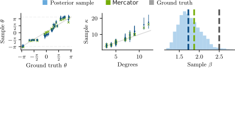
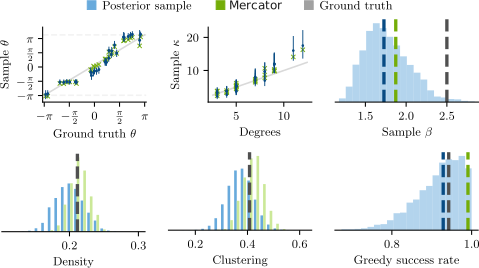
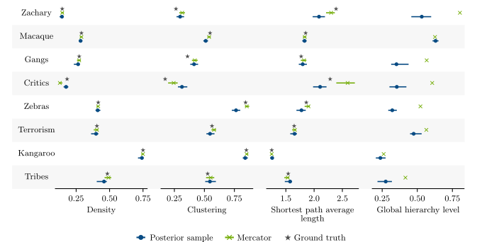
Empirical networks properties
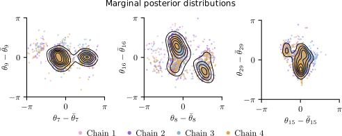
Induced multimodal distribution
Conflicting ground truth model:
A vertex \(v\) is given two positions \(\theta_v^{(1)}\) and \(\theta_v^{(2)}\).
When generating \(G\) with the \(\mathbb{S}^1\) model, each edge probability including \(v\) uses randomly \(\theta_v^{(1)}\)or \(\theta_v^{(2)}\).
Takeaways
- Hyperbolic random geometric graphs reproduce many empirically observed properties.
- Locality \(\implies\) clusters as coarse-graining;
- Bayesian approach finds error bars and can identify multiple good embeddings.
Paper:
Lizotte, A., Young, J.-G. and Allard A. Symmetry-driven embedding of networks in hyperbolic space. arXiv:2406.10711 (2024).
[Accepted at Communication Physics]

 Antoine Allard
 Jean-Gabriel Young
Synthetic graph of 100 vertices
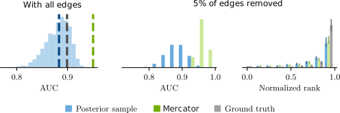
Link prediction is equivalent when sampling
Greedy routing
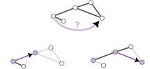
Go to the neighbour closest to the destination.
Model symmetries
The \(\mathbb{S}^1\) model is not identifiable because of graph and space symmetries.
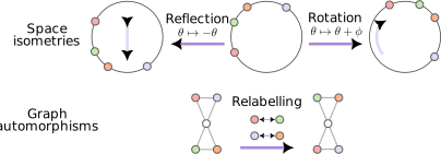
Comparing embeddings requires alignment.